Advanced Curve Fits
In this tutorial, we will cover some of the more advanced features of Yob's Curve Fitting. Our example will determine the apex of a football's trajectory using sparse data.
If you haven’t done so already, you may want to check out the Getting Started tutorial before you continue.
The Data
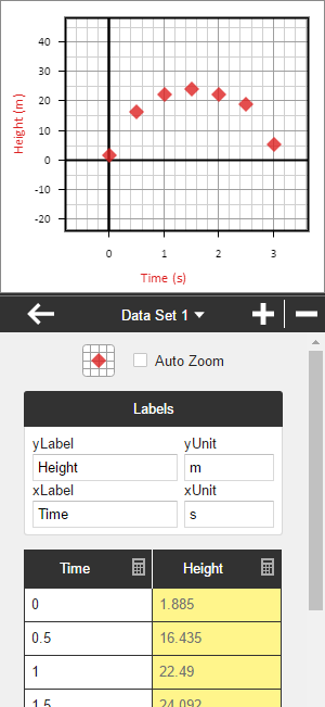
| Time (s) | Height (m) |
|---|---|
| 0.0 | 1.885 |
| 0.5 | 16.435 |
| 1.0 | 22.49 |
| 1.5 | 24.092 |
| 2.0 | 22.289 |
| 2.5 | 19.084 |
| 3.0 | 5.375 |
Copy this data into a new Data Set and set the appropriate labels. If you don't know how do this, you may want to take a look at our Getting Started tutorial to learn how. If all goes well, you should have something like this:
Fitting a Curve
Now, let's go ahead create a new Curve Fit from the Curve Fit menu. First, we will select the Data Set we just created from the Data Source selector since this is the data we want to fit. Then, within the Model submenu, we want select quadratic for the type, which has the form A*x^2 + B*x + C. After doing this, you should see that a curve has been fit to the data:

If you scroll down to the Parameter Output section, you should see the estimated values for A, B, and C. In this model, A represents the vertical acceleration of the football (i.e. acceleration of gravity), B represents the inital velocity of the football, and C represents the inital height.
Using a Custom Model
Since we were trying to find the apex of the football's trajectory, the variables from the default quadratic model don't really help us. To better represent this problem, we need a different version of the quadratic model. The vertex form, or A*(x - H)^2 + K is what we are looking for. Yob doesn't support this model by default, but we can create a custom model to represent the vertex form.
First, select Custom for the model type, then enter A*(x - H)^2 + K into the expression field like so:
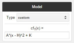
Now the value of H should represent the time that the football reaches the apex of its trajectory, while K represents the height of the apex.
Guess Parameters
It is possible that the Curve Fit didn't quite fit the data as expected, as the following graph illustrates:
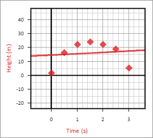
Without going into too much detail, custom models generally need good inital parameter guesses to fit data well. You can set better guesses by checking the Manual Guess check box within the Guess Parameters section, then changing the parameter values below. For this data, we recommend setting A to -9.8, H to 1.5, and K to 25. (You might not even need to finish entering the guesses before the curve snaps into place.) To learn more about guess parameters, check out the section on it here in the Curve Fit Reference.
Alternative Fitting Methods
Up until this point, we've largely ignored the Method selector in the Curve Fit menu. For most data sets you will encounter, the default OLS, or Ordinary Least Squares method will work just fine. However, there are some situations where an alternative method would be preferred. Consider the following data for example:
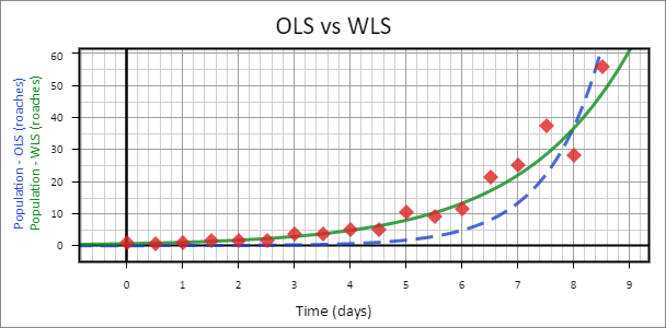
This is a good example of data that is better fit by WLS, or Weighted Least Squares. WLS makes the assumption that error increases with the dependent variable, where as OLS assumes that overall error remains constant. Recognizing when to use alternative methods like this can make a big difference. For more information on the different fitting methods, check out the Curve Fit Reference - Regression Methods.